The Ultimate Tutorial on Leveraging SUMIF in Excel: Techniques and Strategies for Effective Data Analysis

Quick Links

• Use SUMIF For a Single Cell Range
• Use SUMIF With Number Criteria for Multiple Ranges
• Use SUMIF With Text Criteria for Multiple Ranges

Adding numbers together in Microsoft Excel is a basic calculation that can use the SUM function. What if you want to add those values but only if they meet certain conditions? This is when the SUMIF function comes in.

With SUMIF, you can add the values in the cells you specify as long as they meet specific criteria. Maybe you want to find the total sales but only for certain products or the total revenue but only for particular locations.

If your Excel sheet is set up in a way that your calculation isn’t easily determined, the SUMIF function and its formula can help.

Use SUMIF For a Single Cell Range

The syntax for the function is

    `SUMIF(cell_range, criteria, sum_range)`

where the first two arguments are required. Because sum_range is optional, you can add numbers in one range that correlate to criteria in another.

To get the basic feel of the function and its arguments, let’s start by using a single range of cells without the optional argument.

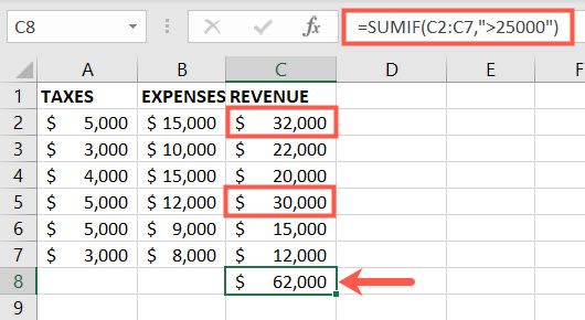
You could add values in a cell range only if they are greater than a certain amount. Enter the following formula, replacing the cell references and criteria with your own.

=SUMIF(C2:C7,”>25000”)

This formula adds the numbers in the cell range C2 through C7 only if they are greater than 25,000.

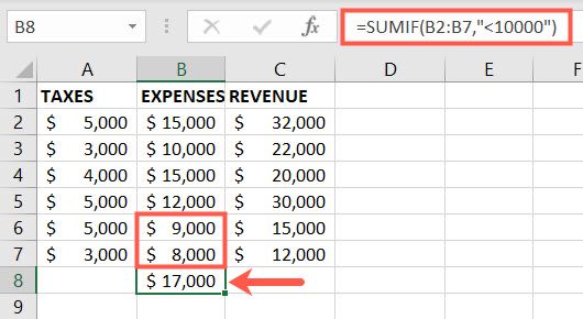
On the flip side, you can add numbers that are less than a certain amount using this formula:

=SUMIF(B2:B7,”<10000”)

This adds the numbers in cells B2 through B7 only if they are less than 10,000.

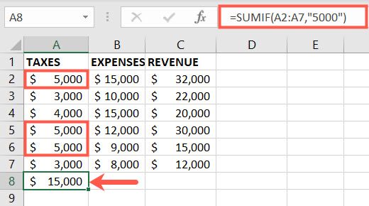
For one more example, you can add numbers that are the same amount with this formula:

=SUMIF(A2:A7,”5000”)

This adds the numbers in cells A2 through A7 only if they are exactly 5,000.

Use SUMIF With Number Criteria for Multiple Ranges

Now let’s put that conditional argument to work, sum_range. Here we’re calculating expenses and revenue. With SUMIF, we can calculate the revenue for locations whose expenses meet our criteria and vice versa.

Related: How to Create Expense and Income Spreadsheets in Microsoft Excel

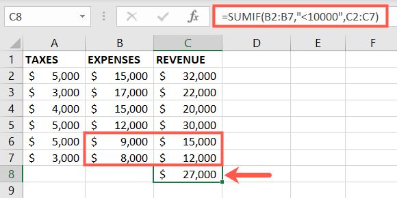
With this formula you can add the revenue in cells C2 through C7 only if the expenses in cells B2 through B7 are less than 10,000.

=SUMIF(B2:B7,”<10000”,C2:C7)

Using the following formula, you can add the expenses in cells B2 through B7 only if the revenue in cells C2 through C7 is greater than 25,000.

=SUMIF(C2:C7,”>25000”,B2:B7)

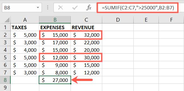
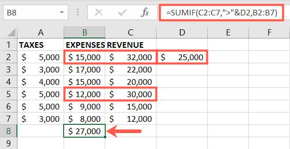
You can also replace the actual value in the formula with one contained in a cell. For instance, this formula adds the numbers in B2 through B7 if the value in C2 through C7 is greater than the value in cell D2.

=SUMIF(C2:C7,”>”&D2,B2:B7)

This formula uses the greater than symbol (“>”) and cell D2 (&D2).

Use SUMIF With Text Criteria for Multiple Ranges

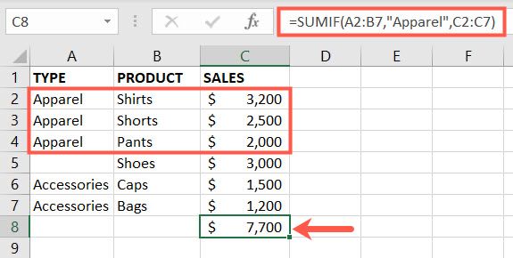
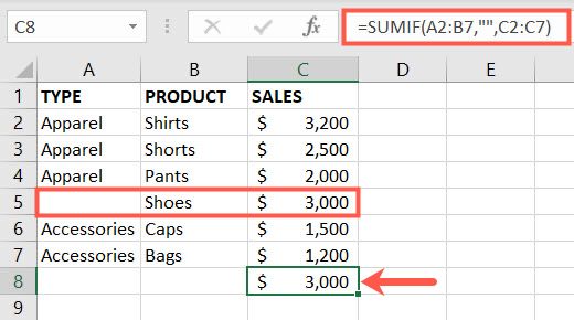
Maybe the values you want to add correlate to text rather than numbers . Here we have types, products, and sales. Using SUMIF, you can add values in the Sales column for products that meet certain conditions in the other columns.

Related: How to Count Cells With Text in Microsoft Excel

In this example, you can add the sales in cells C2 through C7 only if the text in cells A2 through B7 equals the word Apparel.

=SUMIF(A2:B7,”Apparel”,C2:C7)

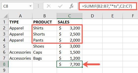
For another example, you can add the sales in cells C2 through C7 for products in cells B2 through B7 that end in “ts.”

=SUMIF(B2:B7,”*ts”,C2:C7)

In this formula, the asterisk (*) is a wildcard representing any letters before “ts”.

One more example uses our Shoes product whose Type is blank.

=SUMIF(A2:B7,””,C2:C7)

In this formula the quotation marks are side-by-side with no space between them. This gives us the sales for Shoes as seen below.

The SUMIF function in Excel allows you to take a basic equation and spice it up to fit your needs. It’s super handy when adding numbers isn’t as simple as two plus two.

For additional help, take a look at how to find the function you need in Excel .

Also read: