Step-by-Step Tutorial on Arranging Data Values Within Microsoft Excel

Quick Links

• Let’s Look at an Example

Excel has “Sort A to Z” and “Sort Z to A” features that let you sort values alphabetically or numerically, and a “Custom Sort” feature that lets you sort using multiple criteria. Here’s how to use them.

Let’s Look at an Example

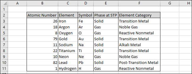
In this example, we have chosen nine chemical elements from the periodic table, and we will sort the data based on the cell contents using the “Sort A to Z” feature and the “Custom Sort” feature.

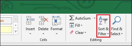
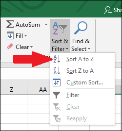
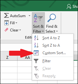
The “Sort & Filter” drop-down is located on the far right of the “Home” tab.

Click here

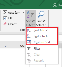
The drop-down has several features listed, but we are focusing on the first three.

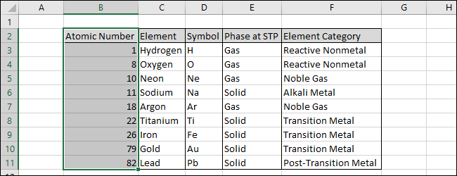
Here is our example data, taken from the periodic table. Each “Element” has information that is unique to it, such as its “Symbol” and “Atomic Number.” But each element also belongs to other categories, such as its “Phase at STP” (i.e., whether it is a solid, liquid, or gas in a room at standard temperature and pressure) and its “Element Category” on the period table.

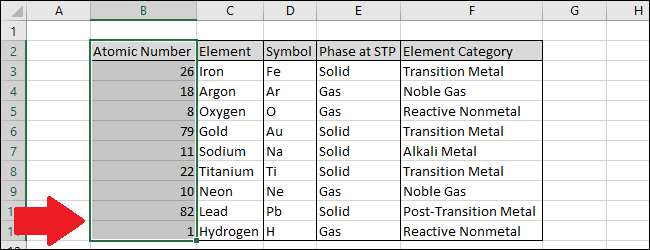
Let’s start simple and sort the data by the “Atomic Number” column. Start by selecting the column (you can include the header row if your data has one).

Now navigate to the “Sort & Filter” drop-down and select either the first or second option. In this example, we will sort from the lowest to highest numerical value using the “Sort A to Z” feature.

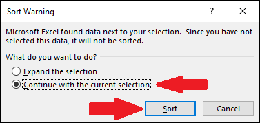
A “Sort Warning” box will appear if there are other columns of data Excel thinks you might want to include in your sort. Let’s examine the results of the “Continue with the current selection” option, first. Click that option and press the “Sort” button.

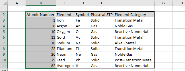
You can see that the “Atomic Number” column has been sorted from lowest to highest, but that the corresponding information in the other columns has not changed. This could be problematic if you wanted to sort all of the columns. So, before moving on, look at some of the rows to see if they make sense. In this case, it is obvious that the other columns have not been sorted because Hydrogen, the element with the lowest “Atomic Number,” is shown as having the “Atomic Number” of Lead.

Now let’s try the other option to see how it works. Select the “Expand the selection” option and click the “Sort” button.

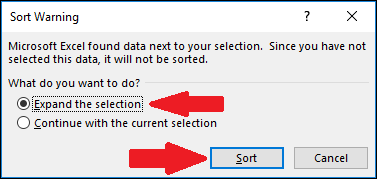
You can see that the data in the “Atomic Number” column has been sorted and the data in the other rows followed it. (You could also just highlight all the data and Excel won’t show a “Sort Warning” box.)

Now let’s see how we can use the “Custom Sort” feature to sort the data by several different columns at once.

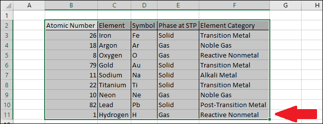
Select all of the data, include the header row if your data has one.

Now navigate to the “Sort & Filter” drop-down and select the “Custom Sort” command.

This brings up the Sort window.

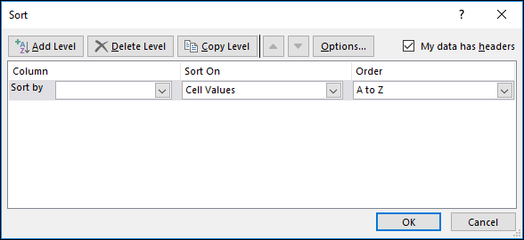
We will sort our data first by using the “Phase at STP” column so that all of the gasses will appear higher on the list than the solids. Select the “Phase at STP” column.

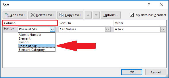
Now press the “Add Level” button.

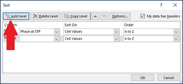
A new level appears. Note that the level says “Then by.” This means it will be the second column used to sort the data. We will choose the “Element Category” as the second level so that the gasses are sorted by their category and noble gasses will appear higher on the list than the reactive gasses. Select the “Element Category” column.

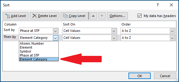
Notice that there are other options. Let’s take a look at the “Sort On” drop-down options. There are a variety of options, but we will use the “Cell Values” option.

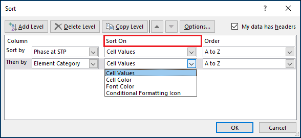
Add another level by pressing the “Add Level” button again.

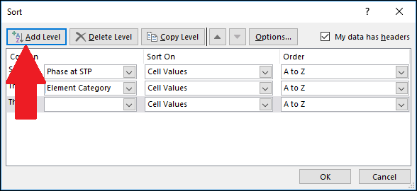
Select the “Element” column. This means that the “Element” values in each “Element Category” will be sorted alphabetically so that the noble gas Argon will come before the other noble gas, Neon.

Let’s look at the “Order” drop-down. There are a few options, but for this example, we will choose the default “A to Z” sort order.

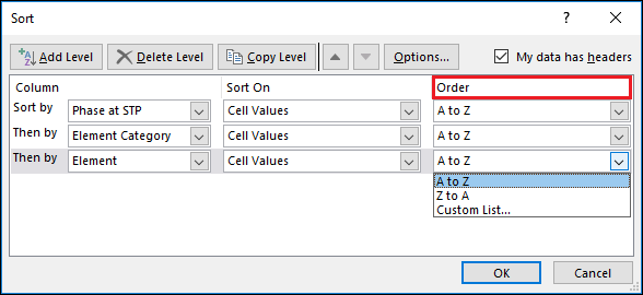
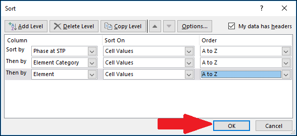
You can add as many levels as will fit in the “Sort” box. When you’re finished, click the “OK” button.

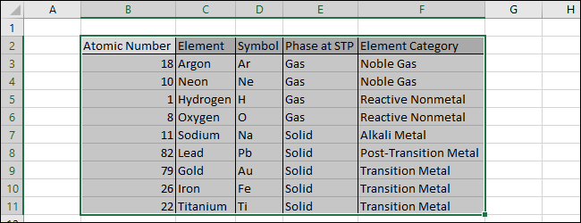
The data has been successfully sorted. The sort order was first by “Phase at STP,” then “Element Category,” and then by “Element.” You can see that the “Phase at STP” column is sorted alphabetically and within each “Phase at STP” type, the “Element Category” values are sorted alphabetically. And finally, the “Element” values are sorted alphabetically within each “Element Category” type.

Note: Be sure to select all of the columns you need when preparing to sort your data. Excel will not warn you that you may be overlooking columns when you use the “Custom Sort” feature.

Also read: