Master Microsoft Excel: A Comprehensive Guide with 12 Tricks for Correcting Faulty Formulas

Quick Links

• Check You’ve Used “=”
• Use the Correct Number Formatting
• Avoid Circular References
• Turn on “Automatic Calculation”
• Avoid Formatting Within Your Formula
• Review Your Formula for Extra Characters
• Close All Parentheses
• Check Your Referenced Cells
• Use Excel’s Function Guide
• Only Use Double Quotes for Text
• Don’t Nest More Than 64 Functions
• Don’t Try to Divide by 0

Excel formulas can be magical things, saving you time and combining vast arrays of data to speed up your number crunching. However, sometimes, the smallest error within your formula can frustratingly limit the quality and validity of your results. Let’s take a look at the ways you can overcome these errors.

1. Check You’ve Used “=”

The first part of an Excel formula must contain the “equals” symbol. This tells Excel that you are creating a calculation within your spreadsheet. If you don’t use “=”, Excel thinks that you’re simply inputting data into the cell you’re typing in, so it won’t perform any calculations.

2. Use the Correct Number Formatting

Excel allows you to define the type of data you are inputting into a cell. In the Home tab on the ribbon, head to the “Number” group and click the drop-down arrow.

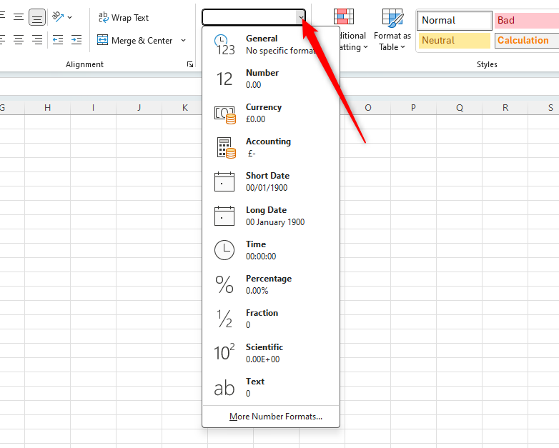
For the formula to work, ensure the correct number formatting is selected.

• “General” works well, as it copies the formatting of other cells if you’re referencing those in your formula—for example, if you’re referencing two cells containing a currency, you’ll probably want your result to be the same currency, and the “General” number format does this automatically.
• “Number” is another good option. However, bear in mind that this generally gives a result with two decimal places, so you might want to change the number of decimal places after you have completed your formula.

Most other number formats are good choices depending on what type of result you’re looking for. However, you must avoid “Text,” as this tells Excel that you’re placing text into the cell, so it won’t see your input as a formula. This number format will result in what you type being displayed in that cell.

3. Avoid Circular References

When you press Enter after typing your formula, Excel might tell you that you have included circular references within your formula.

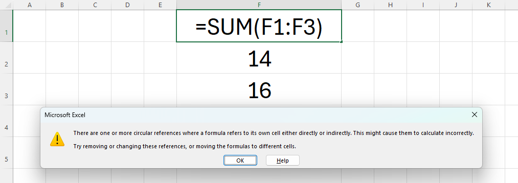
This means that, within your formula, you have referenced the cell you’re typing in. In the case above, the formula typed into cell F1 references the cell itself, which means that Excel cannot properly calculate what you’re telling it to do. The best way to fix circular references is to close the warning that appears (click “X” or “OK”), press Ctrl+Z to undo what you just input, and type the formula again in a different cell.

4. Turn on “Automatic Calculation”

Another reason why your formula might not be working properly is that Automatic Calculation is turned off. If this is the case, the formula result will not automatically update when you change the data referred to in your formula.

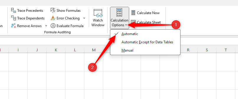
To correct this, first, select the cell where you’re inputting your formula. In the “Formulas” tab on the ribbon, go to the “Calculation” group, click the drop-down arrow next to “Calculation Options,” and make sure the “Automatic” option is checked.

If you want to ensure Automatic Calculations are turned on for your whole workbook, click “File” (top left corner of your Excel window), and then “Options” (bottom left corner of the menu that opens). In the window that opens, go to the “Formulas” menu and ensure “Automatic” is checked under the “Workbook Calculation” option.

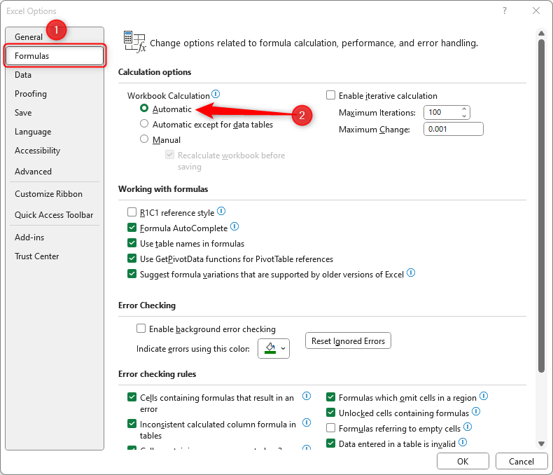
These steps will tell Excel that you want it to recalculate if you change the data referred to in your formula.

5. Avoid Formatting Within Your Formula

As we stated in point 2, by default, if you’re creating a formula that references a cell with a pre-defined number format, like a currency or a percentage, your formula will automatically copy the number formatting.

In the example above, the person typing the formula wants to add two monetary values together within their formula. This can cause problems as certain symbols have certain functions within formulas. Instead of typing the currency symbols within their formula, they should use the accounting number format in the cell that they are typing, as this will automatically format their result to include the dollar symbols.

6. Review Your Formula for Extra Characters

This might sound obvious, but simply reviewing your formula manually can often highlight any issues straightaway. Look out for extra characters that shouldn’t be there, spaces within cell references, or numbers that you might have typed accidentally when constructing your formula.

After having done this, you can also tell Excel to check for any errors for you. Click the “Formulas” tab on the ribbon, and in the Formula Auditing”group, click “Error Checking.”

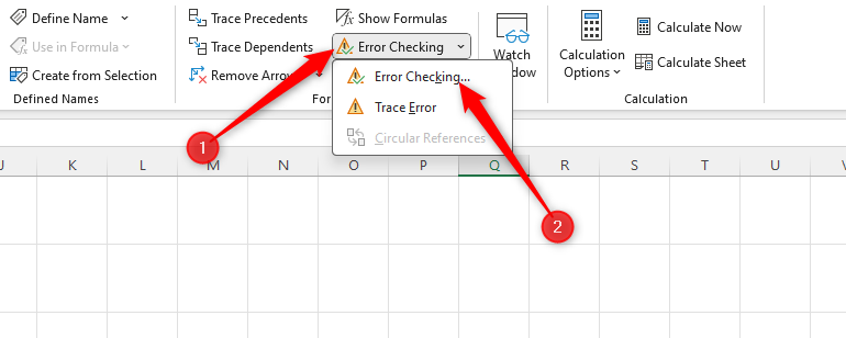
This will highlight most problems with your formulas.

7. Close All Parentheses

If you have a formula with several arguments, you will have used several opening parentheses.

=IFERROR**(AVERAGE((TAKE(Ratings!FZ4:INDIRECT(**”Ratings!GA”&$AI$9

In this formula that we have started to type, there are five opening parentheses. As a result, we need to ensure that each argument created by an opening parenthesis is completed, so we would need five closing parentheses to ensure our formula is correctly constructed.

8. Check Your Referenced Cells

Does your formula’s result appear incorrect? If so, check that you have referenced the correct cells.

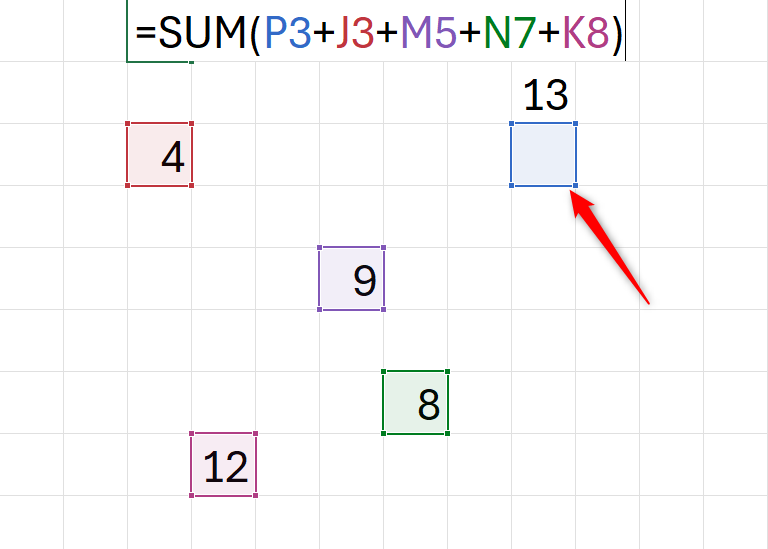
If you double-click on the cell containing your formula, Excel will color code the references within the formula. By doing this, we can quickly see if any of the cell references are incorrect. To fix this, simply drag the colored cell reference to the correct cell, and the formula will automatically update.

9. Use Excel’s Function Guide

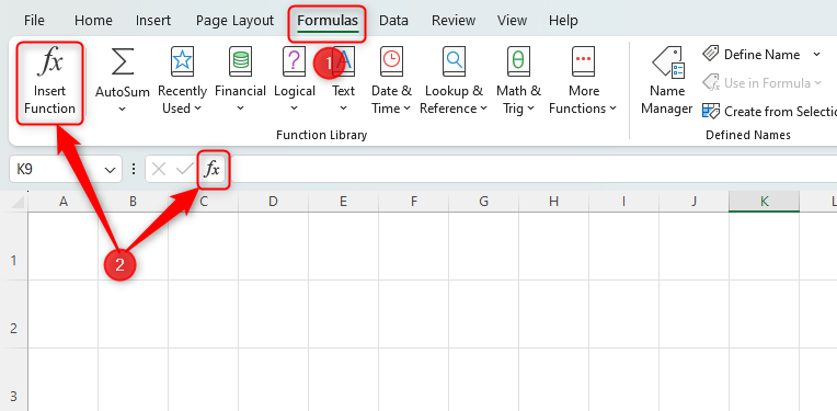
A good way to overcome frustrating formula errors is to use Excel’s function guide instead of typing the formula manually. In the “Formulas” tab on the ribbon, click “Insert Function”. Alternatively, click the same symbol next to your formula bar.

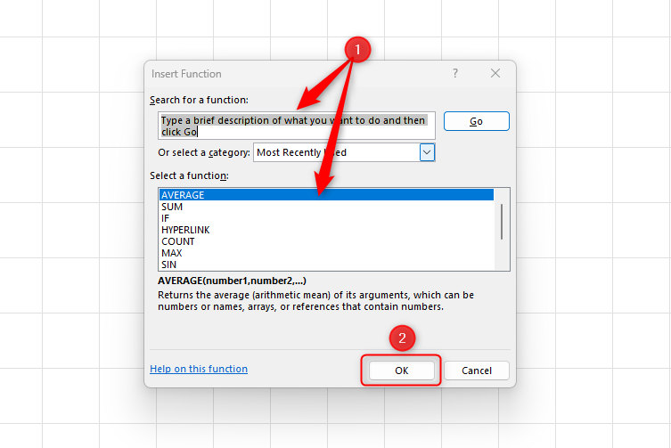
In the dialog box that opens, you can either type the name of the function you’re looking to use in the “Search For A Function” box, or select from the list below. Once you’ve found the correct function, click ‘OK’, and Excel will take you through the steps to ensure your formula is correctly input.

10. Only Use Double Quotes for Text

If you include double quotes within your formula, Excel will see this as text to include in the result.

Here, we have used the IF function .

In this example, if cell S9 is equal to 2, the formula will return the word “Yes”. If it’s not equal to 2, the formula will return “No”. This is because we have used double quotes around these two words to tell Excel to add text to the cell containing the formula . So, if your formula doesn’t work, make sure you have not used double quotes accidentally.

11. Don’t Nest More Than 64 Functions

If you use functions within arguments in Excel, you are nesting your formula.

In this example, we are nesting the AVERAGE and SUM functions within the IF function.

=IF(AVERAGE(A1:A10)>100,SUM(B1:B113),”FAIL”)

Excel allows a maximum of 64 nested functions within one formula. If you use more, the formula will not work.

12. Don’t Try to Divide by 0

Have you ever tried to use a calculator to divide by zero? If so, you’ll know that it returns an error. This is because it’s impossible to divide by 0. If you try to do this in Excel, you’ll see

#DIV/0!

In this example, Dick’s profit per hour returns the above error, because he hasn’t worked any hours.

To get around this, you would use the IFERROR function to hide the error and insert an alternative value or return a blank cell.

Now that you know how to troubleshoot errors in Excel formulas, you can also evaluate formulas , which can be useful if you want to break down a formula that someone else has typed.

Also read: