Ditch the Expensive Software - Mastering Project Management with Just Excel

Quick Links

You might be tempted to browse the web for top-of-the-range programs to help you with your project management. But stop—I’m going to talk you through some of Excel’s tools that you can use and reuse to efficiently manage your project without having to fork out for expensive software.

Use Drop-Downs

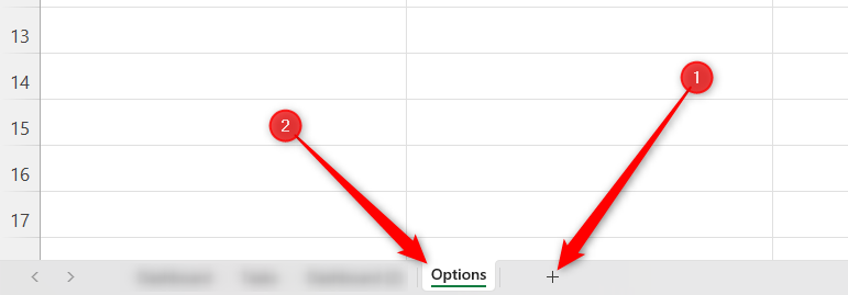
Drop-downs are a great way to speed up your work processes, and make your project management system more professional. First, create the options to appear when you click a drop-down cell. Click the “+” at the bottom of your workbook, and double-click the new tab to rename it Options.

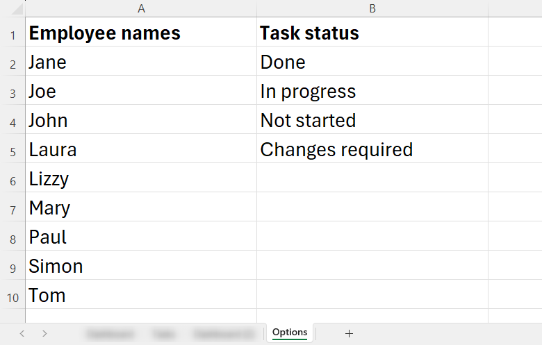
I need employee names and task status as drop-down options in my workbook, so I’ll create the lists for these here.

Now, create another sheet where the tasks will be managed and rename it Tasks.

After creating a table with the task names on the left and an appropriate header at the top, select the cells that will contain the first drop-down with the options you just created on your Options sheet.

Kanto Player Professional

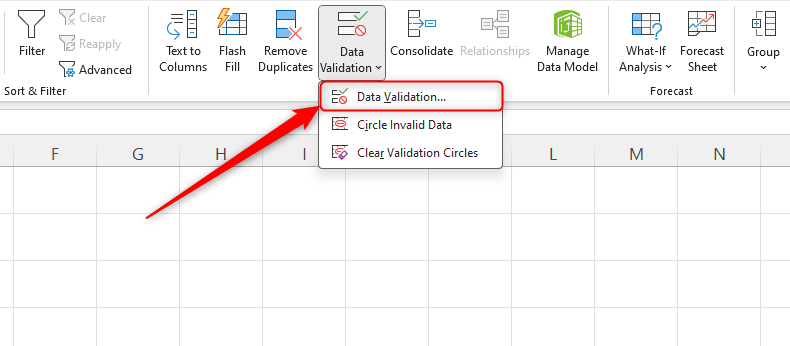
Next, in the Data tab on the ribbon, click “Data Validation.”

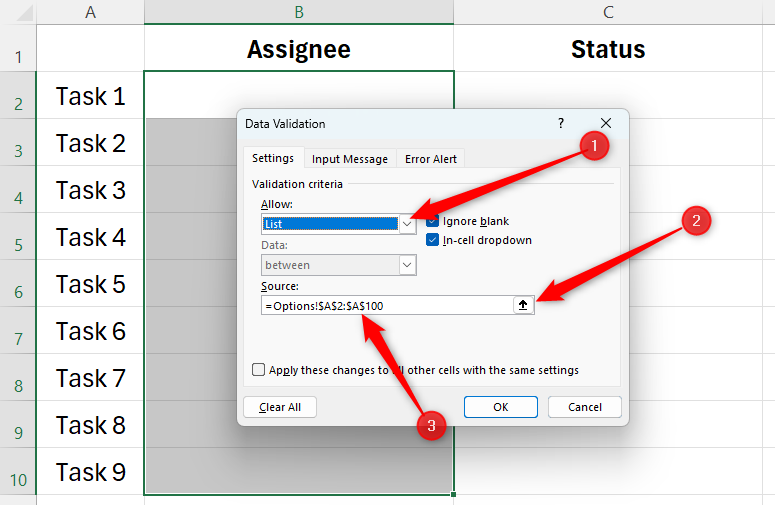
In the Allow field of the Data Validation dialog box, choose “List.” Then, click the Source field arrow, head to your Options sheet, and select the appropriate values for this drop-down. In my case, it’s the values underneath the Employee Names heading, and their cell references will then show in the dialog box field. Even though the list of names runs from A2 to A10 on our Options sheet, I’ve selected A2 to A100 for our data validation, as this means any new names I add to the list will also be picked. Finally, click “OK.”

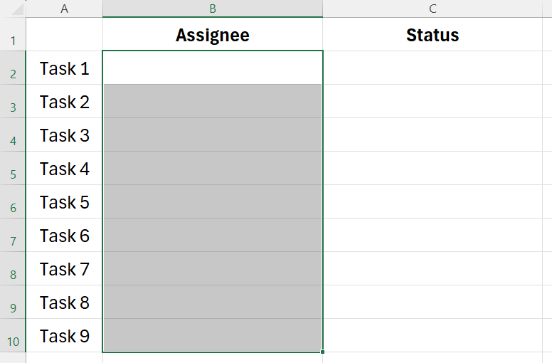
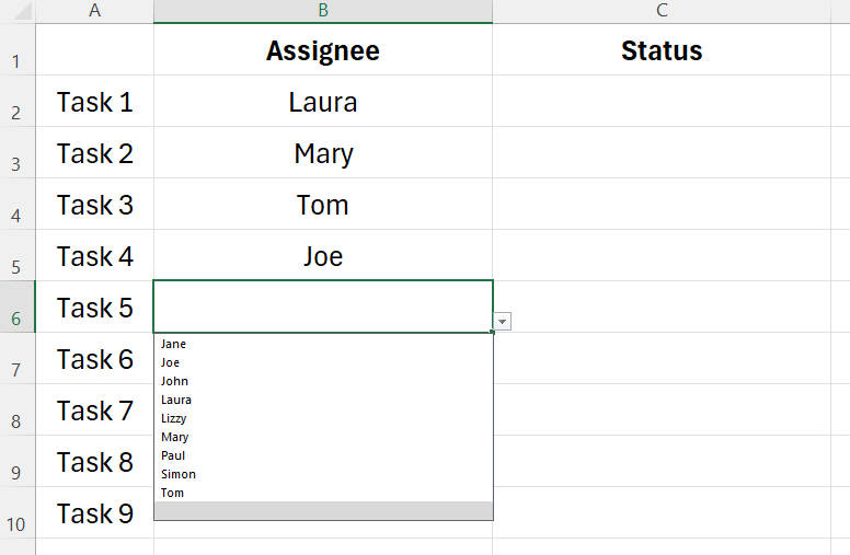
You will then see the list of names appear when you click any cell in the Assignee column.

DLNow Video Downloader

Now, repeat the process for the Status column, and anytime you want to add a drop-down list to your workbook, you can use and hide your Options sheet to create the choices.

CollageIt Pro

Create Gantt Charts to Track Progress

A Gantt chart is a simple but effective table that shows you what task needs to be done in a project and when they need to be completed.

Excel has tools for creating simple Gantt charts , but they are less adaptable than those created from scratch. Keep reading to see how to create a more dynamic Gantt chart.

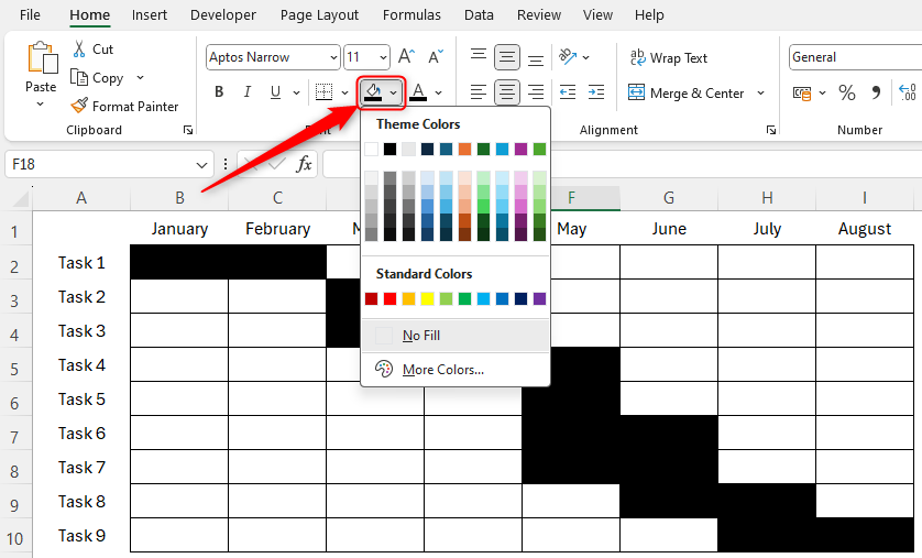
Step 1: Mark Your Timings Manually

Click “+” at the bottom of your workbook to create a new sheet, and call it Timing. On this new sheet type the tasks’ names on the left and the months at the top. Next, map out your proposed timings using manual color fill. It doesn’t matter what color you use, as this will be covered up later when we add more settings. Select the first cell you want to color, hold Ctrl, and then select the remaining cells. Then, go to the “Fill Color” drop-down in the Home tab on the ribbon and choose a color.

Step 2: Color the Cells According to Progress

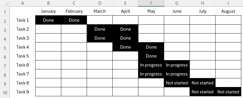
I now want to color the cells according to their status. I’ll do this by referring to the status I set for each task on the Tasks sheet set up in the section above. In the first colored cell of your Gantt chart, use the VLOOKUP formula :

=VLOOKUP(x,y,z)

where x is the cell reference in the chart you’re looking up, y is where Excel should look to find the corresponding value, and z is the column number within the array.

So, here’s what I’ll type into my first Gantt chart cell:

=VLOOKUP($A2,Tasks!$A$1:$C$1000,3)

Because I have used mixed and absolute references (using the $ symbol) within our formulas , I can copy (Ctrl+C) and paste (Ctrl+V) this formula into the other colored cells.

If you use a black color fill, use white font so that you can see the values against the black backgrounds.

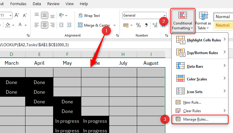
Finally, use Conditional Formatting to color the cells based on the values they contain.

Select all the cells in the Gantt chart, and in the Home tab on the ribbon, click Conditional Formatting > Manage Rules.

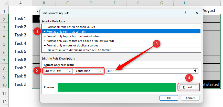
Click “New Rule” in the dialog box that appears, and create the following conditions (after you have set each one, click “OK” to set the next):

For each rule, set the Rule Type to “Format Only Cells That Contain.”
Select “Specific Text” and “Containing” in the first two drop-down boxes.
In the text box, type Done, In progress, Not started, or Changes required for each rule you create (as these are the options in the VLOOKUP for these cells that we created in the previous step).
For each rule, format both the fill color and the text color to be the same—green for Done, yellow for In progress, and so on.

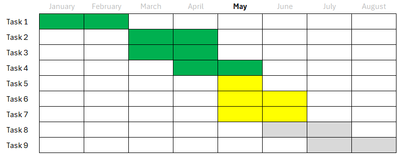
You will then see the relevant Gantt chart cells change color based on their status in the Tasks sheet.

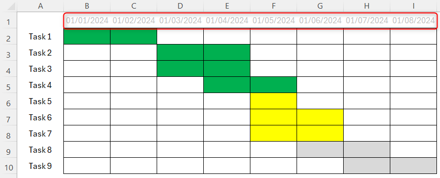
Step 3: Highlight the Current Month

Start by typing the first date of each month in short form where you originally typed the name of the month. So, for example, replace the text in the cell containing January with 01/01/2024. Then, do the same for February, before using AutoFill to complete the remaining months . Doing this tells Excel that these are dates, and not just text. Next, change the font color of these dates to gray.

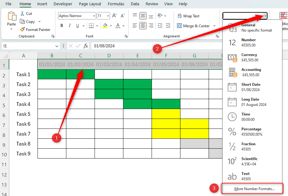
To turn these back into the names of the months, select all the dates, click the Number Formatting drop-down option in the Home tab on the ribbon, and click “More Number Formats.”

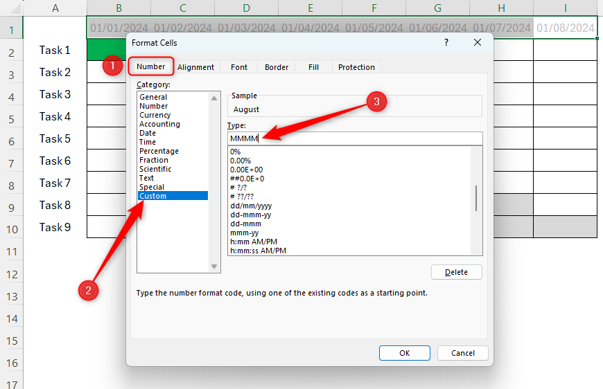
In the Format Cells dialog box, open the “Number” tab, and click “Custom” in the Category list. Then, in the Type field, type MMMM.

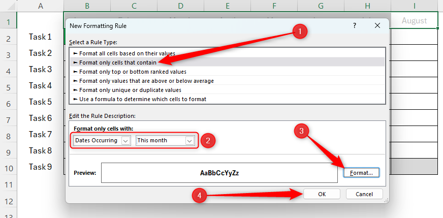
Then, click “OK” to see the result. To now make the current month stand out, select all the months in your Gantt chart, and click Conditional Formatting > New Rule. In the dialog box, click “Format Only Cells That Contain,” select “Dates Occurring” in the first drop-down menu, and “This Month” in the second. Next, choose the formatting you want to use to make the current month stand out, such as black and bold text. Finally, click “OK.”

You now have your completed and dynamic Gantt chart with the progress displayed and the current month emphasized.

/a>

Create a Progress Tracker

Using the Gantt chart created in the steps outlined above, you can now create a progress tracker. You can either do this on the same sheet as where your Gantt chart is located or on a new tab. In my case, I want to show how many squares in our Gantt chart are marked as Done, In progress, Not started, and Changes required, and then calculate an overall progress percentage.

To do this, I’ll need to use the COUNTIF function , which follows this syntax:

=COUNTIF(x,y)

where x is the array to evaluate and y is the criterion to count.

So, for the Done count, we will type

=COUNTIF($B$2:$I$10,”Done”)

$B$2:$I$10—This references the cells in the Gantt chart using an absolute reference (notice the $ symbols).
**”Done”**—Use the quotation marks to tell Excel you’re looking to count the number of times this text string appears in the array.

Then, copy and paste this formula for the remaining details in your progress tracker, changing value y to match the value you’re looking to count.

Next, calculate the overall progress using the following formula:

=SUM(a/(a+b+c+d))

Where a is the number of cells in your Gantt chart containing the word Done, and b, c, and d are the number of cells containing the other status markers. Remember to change the number format of this cell to a percentage.

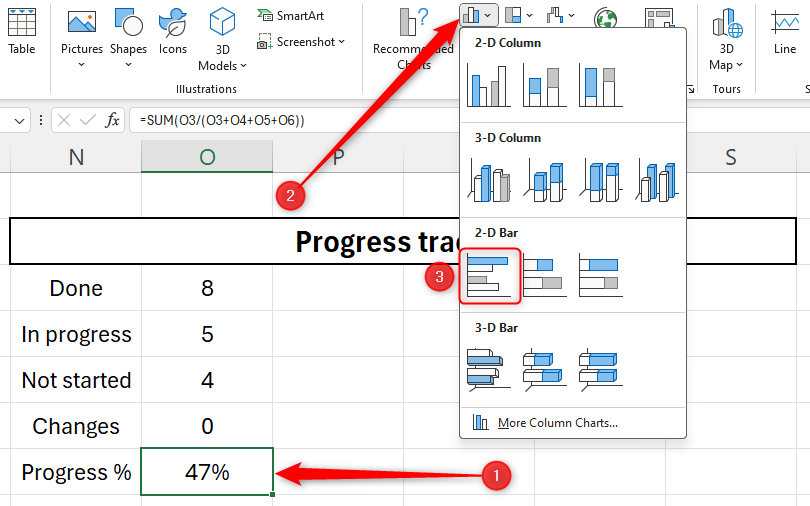
With Screensaver Wonder you can easily make a screensaver from your own pictures and video files. Create screensavers for your own computer or create standalone, self-installing screensavers for easy sharing with your friends. Together with its sister product Screensaver Factory, Screensaver Wonder is one of the most popular screensaver software products in the world, helping thousands of users decorate their computer screens quickly and easily.

With the cell containing the newly calculated percentage selected, in the Insert tab on the ribbon, click the Chart button highlighted below, and select a 2-D bar chart.

Then, format your chart to remove any details you do not require, resulting in a progress bar showing your overall progress.

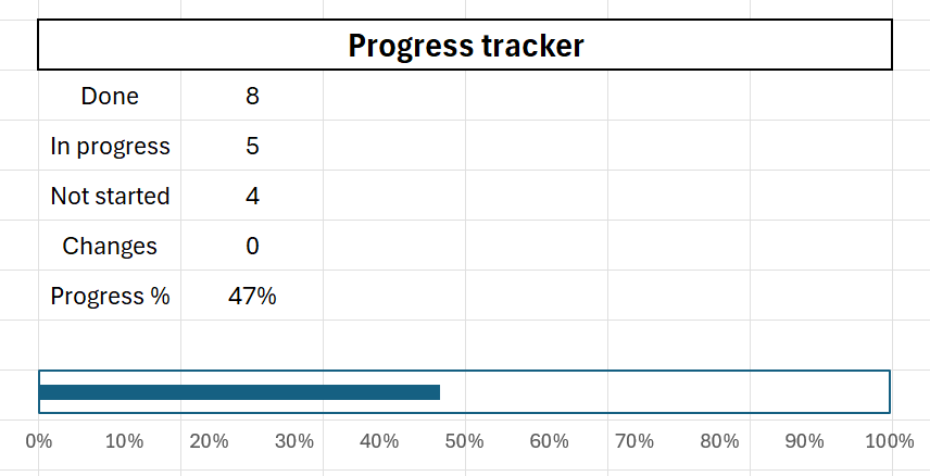
Remove the gridlines to make your progress bar easier to read and look more professional.

Display Due Dates and Time Remaining

As well as tracking your project’s progress, you can also track the time elapsed and time remaining.

1. First, type the start and due date manually using a date format that suits your region. Excel will automatically convert this to a date format, and you can amend the date format if required.

2. Next, add today’s date by typing

=TODAY()

and pressing enter.

3. Third, calculate the days elapsed so far using the following formula:

=SUM(x-y)

where x is the cell containing today’s date, and y is the cell containing the start date. Then, calculate the weeks elapsed by dividing the days elapsed by seven.

4. You can also calculate the days remaining with the following formula:

=SUM(a-b)

where a is the cell containing the due date, and b is the cell containing today’s date. Again, calculate the weeks remaining by dividing the days remaining by seven.

5. Then, create a percentage of the time passed with the following formula:

=SUM(c/(c+d))

Where c is the total number of days elapsed and d is the total number of days remaining.

6. Finally, create a 2-D bar chart using the method described in the previous section.

Now you’ve created the perfect spreadsheet for project management, consider using Excel to help you monitor your budgets !

Windows11

Ditch the Expensive Software - Mastering Project Management with Just Excel