1. Mastering Excel: A Step-by-Step Guide to Revealing Hidden Data

Quick Links

Key Takeaways

First, select your entire worksheet using Ctrl+A (Windows) or Command+A (Mac). Press Ctrl+Shift+9, right-click a cell, and choose “Unhide,” or select Format > Hide & Unhide > Unhide Rows from the ribbon at the top to unhide all rows.

Unhiding all the rows in a Microsoft Excel spreadsheet is as easy as pressing a keyboard shortcut or using a button on the ribbon. We’ll show you how.

How to Unhide All Rows in Excel With a Shortcut

To show hidden rows in your spreadsheet, launch your spreadsheet with Microsoft Excel . Then, access the worksheet in which you have the hidden content.

Select your entire worksheet by pressing Ctrl+A (Windows) or Command+A (Mac). Alternatively, click the “Select All” button in the worksheet’s top-left corner.

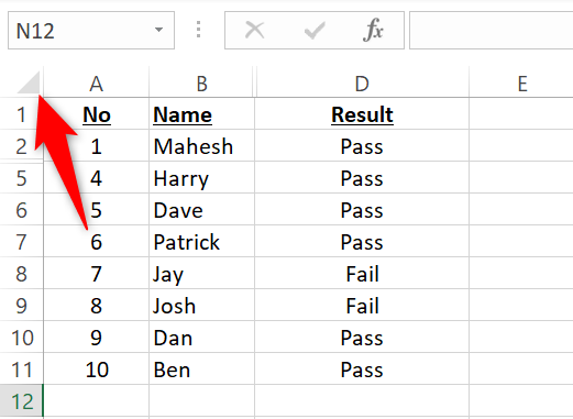
While your worksheet is selected , unhide all rows by using this shortcut: Ctrl+Shift+9. Or, right-click a selected cell and choose “Unhide” in the menu.

WPS Office Premium ( File Recovery, Photo Scanning, Convert PDF)–Yearly

How to Unhide All Rows and Columns in Excel

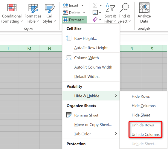
Alternatively, in Excel’s “Home” tab in the ribbon, click the Format > Hide & Unhide > Unhide Rows option. This also works for

Excel will make all your hidden rows visible again in your spreadsheet. You’re all set.

Project Manager - Asset Browser for 3Ds Max

How to Unhide Specific Rows in Excel

To reveal only specific rows while keeping all other hidden items invisible, use the following method.

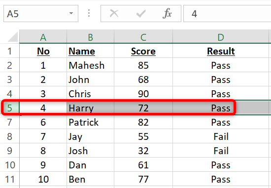
To unhide a specific row, click the header of the row that’s above your hidden row. For instance, to unhide row

`6`

, click the header for row

`5`

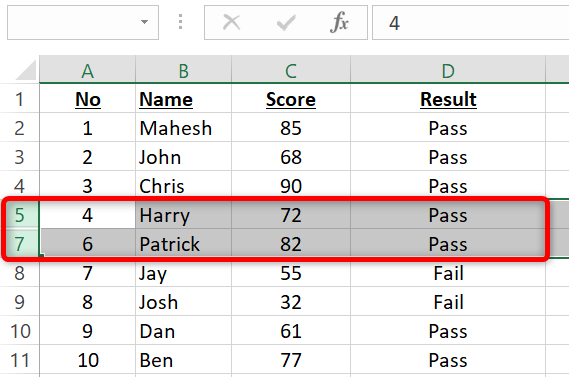
ZoneAlarm Pro Antivirus + Firewall NextGen

Now, press and hold down the Shift key on your keyboard and click the header of the row that’s beneath your hidden row. In the above example, you’ll click the header for row

`7`

(while the Shift key is held down).

You hold down Shift and click a row header because doing so selects all the rows between your clicked items. This selects your hidden content as well, which you’ll unhide in the following step.

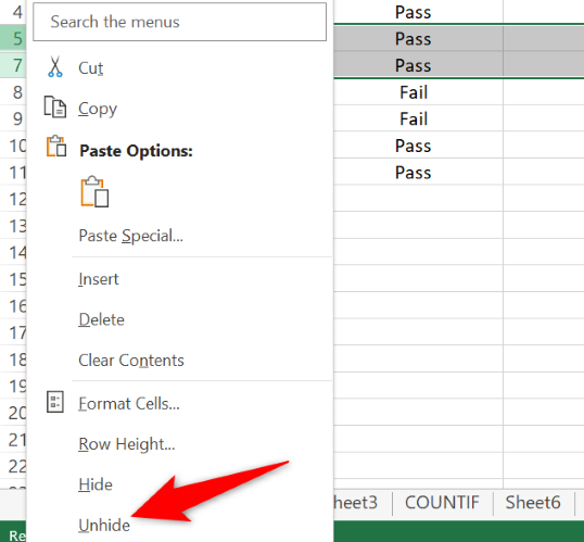
Right-click the header of a selected row and from the open menu, choose “Unhide.”

And that’s it. Excel has unhidden your selected content, and you can now work with it the way you want .

Want to unhide all of your Excel columns too? Check out our guide.

Windows11

1. Mastering Excel: A Step-by-Step Guide to Revealing Hidden Data